Introduction

On March 11, 2020, the World Health Organization (WHO) declared COVID-19 to be a pandemic (WHO, 2020). Since then, the pandemic has spread worldwide disrupting economies and society. In order to control the spread of the virus, countries have imposed lockdowns that have restricted economic and social activities and movement of people. There is considerable divergence across countries in terms of the intensity and timing of stringency measures. For example, Sweden had a relaxed approach to stringency with minimal economic and social restrictions (Ferraresi et al., 2020a) while many other countries including India imposed a stringent lockdown early on in the pandemic. While lockdowns and stringency measures are intended to save lives by minimizing contact, these measures have a considerably harsh effect on the economy and livelihoods of people. One of the challenges of the COVID-19 pandemic has been to find ways to save lives and livelihoods. The question of how stringency measures affect the trajectory of the pandemic is therefore of interest.

  The literature over the last year has investigated various aspects of the relation between lockdown stringency and the trajectory of the pandemic as well as its impact on the economy. Studies have examined determinants of stringency measures identifying variables such as political stability, level of development, and degree of decentralization (Ferraresi et al., 2020a). Other studies have examined the impact of alternative reopening strategies on economic recovery (Demirguc-Kunt et al., 2020). The issue of whether lockdown measures can contain the spread of the virus (Askitas et al., 2020; Mitra et al., 2020) and the degree to which they are effective have also been studied (Ferraresi et al., 2020b; Thayer et al., 2021). The objective of this article is to track the trajectory of the pandemic in India in the two-dimensional space, obtain a composite index of the pandemic and examine its relation to the stringency index.

  A national-level lockdown was imposed in India on March 25, 2020. On the eve of the lockdown, India had 536 coronavirus cases and 10 deaths due to the disease. The Oxford COVID-19 Government Response Tracker (Hale et al., 2020) which calculates the Stringency Index, rated the lockdown as being the most stringent among countries and gave it a rating of 100 on 100. The initial period of the lockdown was for 21 days which was extended in three phases until May 31, 2020. During this period, the relative spread of coronavirus was contained, but as restrictions began to be eased from June 2020 when the unlock phase began, the disease spread rapidly. By mid-September 2020, India had reached the peak of the first wave with nearly 100,000 new coronavirus cases daily and over 1,000 daily deaths. Subsequently, even as unlock measures continued, cases went down and by mid-February 2021, daily new cases were less than 10,000 and daily deaths were less than 100. But from mid-February 2021, a slow increase in cases was observed that ultimately led to an intense second wave of the pandemic in April 2021 with nearly 400,000 daily cases in April–May and over 3,000 daily deaths.

  To examine the relationship between lockdown stringency and the trajectory of the pandemic in India, data on daily observations from March 25, 2020, to May 15, 2021, on six dimensions of the COVID-19 pandemic in India are obtained from Worldometer (Worldometers.info1). For the corresponding period, daily observations on the stringency index are obtained from the Oxford COVID-19 Government Response Tracker (Hale et al., 2020). Using the method of principal component analysis (PCA) for dimensionality reduction, we are able to construct a composite measure of the pandemic. The graphical representation of the score plot in the two-dimensional space enables us to clearly identify four phases in the trajectory of the pandemic. Correlations between the stringency index and the pandemic index are obtained corresponding to the grouping of observations of the trajectory into four phases. While a negative and statistically significant relationship is established between the pandemic index and the stringency index for the entire period of the study, the phase-wise analysis enables us to better understand the relation between the pandemic trajectory and stringency measures. In particular, the decline in the pandemic index even as the stringency index declined in the third phase and the sudden onset of the second wave with a sharp rise in the pandemic index and the corresponding rise in the stringency index in the fourth phase offer insights into managing the future trajectory of the pandemic as well as design of appropriate stringency measures. The understanding gained from the experience of the first two waves of the pandemic is crucial to the design of policies for containment and management of the pandemic. Tracking new epidemiological variants of the virus for their transmissibility has a vital role to play in managing the future trajectory of the pandemic while stringency measures imposed at a geographically localized level rather than a national level may be a more feasible way to balance lives and livelihoods.

  The article is organized as follows. The second section contains a description of the data and methodology. In the third section, we discuss the results while section four presents an analytical discussion. The fifth section summarizes and concludes.

Material and Method

Data

During the course of the COVID-19 pandemic, data on different dimensions of the pandemic such as total number of cases, daily new cases, daily deaths, and positivity rate have been closely examined to get an understanding of the magnitude and scale of the pandemic. Some of these data relate to cumulative numbers while others are daily figures giving the changes in the scale of the pandemic from day to day. Given that these dimensions reveal different facets of the pandemic, one of the objectives of the study has been to use statistical techniques for dimensionality reduction using the data that are available on the many dimensions of the pandemic. The study is based on daily data from March 25, 2020, to May 15, 2021, on six such dimensions relating to the pandemic, that is, total number of coronavirus cases (total cv cases), total number of deaths (total cv deaths), active cases, daily new cases, daily deaths and daily recovered that are available from Worldometer website (Worldometers.info¹). Data on stringency are obtained from the Oxford COVID-19 Government Response Tracker’s Stringency Index (Hale et al., 2020).

  The time series plot of the variables is given in Figure 1. Total coronavirus cases and total deaths are cumulative figures and show an increase although the rate of increase slowed down after mid-September. The remaining four variables show a peak in mid-September and thereafter a decline. All the curves show a sharp vertical spike in April 2021 in the second wave of the pandemic. Due to misreporting and delays in reporting, estimates are sometimes revised when data are made available, leading to bunching of numbers that can be seen as outliers in the plot of variables in the data set.

Figure 1. Time Series Plot of Variables Using Observations from March 25, 2020, to May 15, 2021

Source: Authors’ own (based on data obtained from Worldometer; Worldometers.info¹).

Principal Component Analysis

PCA and factor analysis are multivariate statistical techniques that are used for the purpose of reducing dimensionality of a set of observed variables. However, the two techniques differ from each other in many ways and one of the main differences is that while factor analysis is based on an explicit model, PCA makes no such assumption (Jolliffe, 2002). The basic idea underlying the model in factor analysis is that there are latent factors or unobservable factors underlying the observed variables in the data set. In factor analysis, the model seeks to express the set of observed variables in terms of a smaller set of hypothetical variables that are called latent constructs or factors. The choice between the two techniques depends primarily on the purpose of the study. While both techniques are based on the correlations among the observed variables for dimensionality reduction, factor analysis is an appropriate technique if the aim is to specify a model in order to obtain latent constructs or factors that may be accounting for the variation in observed variables. But if the aim of the study is to reduce the set of correlated observed variables into a smaller set of dimensions with a minimum loss of information, then PCA is an appropriate technique. In this study, we use PCA since the objective is to reduce dimensionality to track the trajectory of the pandemic in a smaller subspace while accounting for as much of the variance in the data on the six dimensions relating to the spread of coronavirus.

  If a data set has many dimensions, then PCA can be used to compress data into a smaller number of dimensions while retaining as much statistical information as possible (Anderson, 1958). This is done by obtaining summary measures called “principal components” which are linear combinations of the observed variables (Jolliffe, 2002; Jolliffe & Cadima, 2016). These principal components (PCs) are ordered in terms of their variance and they are uncorrelated with each other.

  Suppose the data set consists of n observations on p variables, X₁, X₂, … X_p. The principal components are obtained as exact linear combinations of the observed variables as given in Equation 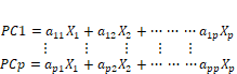(1).

   ⁽¹⁾
                                                                                

The linear combinations PC1, PC2, … PCp are called the principal components. The a_ij’s in Equation (1) represent the weights in the linear combinations of the variables and are given by the eigenvectors of the covariance matrix. Obtaining the linear combinations or principal components thus involves solving an eigenproblem for the covariance matrix of the data set. The covariance matrix for the data which are a p × p symmetric matrix has exactly p real eigenvalues λ₁, λ₂, ... m_p and the corresponding eigenvectors form an orthonormal set of vectors. The eigenvalues λ₁, λ₂, ... λ_p are sorted from largest to smallest and the corresponding eigenvectors sorted accordingly. The principal components are ordered so that the first principal component has largest variance given by the largest eigenvalue followed by the second principal component with the second largest eigenvalue and so on. The principal components successively maximize variance and have the property that they are uncorrelated with each other. The elements of the eigenvector are called loadings and represent the contribution made by each variable to a particular component.

  The principal component scores are the values taken by each observation for any given principal component. The trace of the covariance matrix gives the sum of the variances of the p variables in the data set. This equals the sum of the variances of all p principal components.  The proportion of variance explained by the jth PC is thus given by  

  If the variables are standardized so that they have zero mean and unit variance, then the covariance matrix of the standardized variables is the correlation matrix of the original variables. The coefficients of the linear combinations are given by the eigenvectors of the correlation matrix. The trace of the correlation matrix equals the number of variables p in the data set. For a correlation matrix PCA, the sum of the variances of all p principal components equals p, that is,  and the proportion of variance explained by jth PC is λ_j /p.

  If the original variables are highly correlated then PCA can be used successfully for dimensionality reduction. The decision on the number of principal components to be retained without an unacceptable loss of information is a subjective decision (Rea & Rea, 2016). In general, the rule of thumb is to retain those components which cumulatively account for say 70% or 90% of the variation. Other methods include using a Scree plot (Cattell, 1966) which is a line graph that plots the eigenvalue of each component against the component. A steep fall in eigenvalue of a component that gives the graph an “elbow” shape is used to decide on the number of components to be retained. In correlation matrix PCA, the Kaiser rule is to retain only PCs that have an eigenvalue greater than one (Kaiser, 1960).

  Many studies have used epidemiological and econometric models of the pandemic (Thayer et al., 2021; Thompson, 2020). The method of PCA can also be used to track the spread of COVID-19 disease (Mahmoudi et al., 2021). By tracking the relative clustering and spread of observations in a lower dimensional space, we can evaluate how the pandemic progressed in the different phases of lockdown and unlock in the economy during the last year.

Results

Trajectory of the Pandemic in the Different Phases of Lockdown and Unlock

Before performing PCA we did a preliminary examination of the data set and some tests to check the suitability of the variables for PCA. The Pearson’s correlation coefficients between the six variables are given in Table 1. All the coefficients are high and statistically significant.

Table 1. Correlation Coefficients Between Variables Using Observations from March 25, 2020, to May 15, 2021

Source: Authors’ own (based on data obtained from Worldometer; Worldometers.info¹).

Abbreviation: cv = coronavirus.

Note: 5% critical value (two-tailed) = 0.0960 for n = 417.

  To check suitability of the data set for application of PCA, two tests were performed. The Kaiser–Meyer–Olkin (KMO) test is used to check whether the data are suitable for structure detection (Kaiser, 1970; Kaiser & Rice, 1974). The KMO statistic lies between 0 and 1 and if the KMO value is less than 0.50 then we cannot obtain a low dimensional representation of the data. The results are given in Table 2. All six variables have KMO values of more than 0.60 and the overall KMO value is 0.71. Using Kaiser characterization the overall KMO value is in the “middling” range.

Table 2. Estimates of Kaiser–Meyer–Olkin Measure of Sampling Adequacy

Variable	KMO
Total coronavirus cases	0.6395
Daily new cases	0.6987
Active cases	0.7005
Total coronavirus deaths	0.6026
Daily deaths	0.9349
Daily recovered	0.7172
Overall	0.7125

Source: Authors’ own (based on data obtained from Worldometer; Worldometers.info¹).

The squared multiple correlations of each of the six variables with all other variables were estimated to see if the variables have strong linear relations with each other. Table 3 gives these results and all these correlations are high and statistically significant and therefore all six variables in the data set can be retained.

Table 3. Squared Multiple Correlations of Each Variable with All Other Variables

Source: Authors’ own (based on data obtained from Worldometer; Worldometers.info¹).

  The first step in performing PCA is to standardize the variables if the variables have different scales/units of measurement. Since we did not standardize the variables, we chose the correlation matrix option in STATA. PCA is performed using the correlation matrix to obtain the eigenvalues and their corresponding eigenvectors. Next, a decision regarding the number of components to be retained for further analysis needs to be made. Since correlation matrix PCA was performed, Kaiser’s rule can be applied, and accordingly, we retain only the first two components that have eigenvalues greater than one (Kaiser, 1960). For further analysis, the component loadings on the retained principal components were examined to see if they gave a useful interpretation in the context of the study. Since this was not the case we rotated the first two components using varimax rotation with Kaiser normalization. In this rotation, while the total variance in the rotated two-dimensional subspace remains the same, the variance is now distributed more evenly among the rotated components. The purpose of rotation is to make component loadings easier to interpret (Jolliffe, 2002). In the unrotated components, the four daily variables loaded with near equal weights and the two cumulative variables had low weights on the first component while the second component had large, small, and intermediate loadings making the task of interpretation difficult. Since we wanted to examine the score plot to track the trajectory of the pandemic in the two-dimensional space and interpret the first two components, rotation was applied to give a clearer interpretation of the components. After rotation, the first component loads high on the daily variables and low on the cumulative variables while for the second component the loadings for the variables are reversed, thus enabling easy interpretation. As the rotated components were found to have loadings with a simpler structure and a clearer interpretation than the original coefficients, we retained these results for further analysis. The results are given in Table 4.

  The top half of Table 4 gives results for variance and proportion of variance and cumulative values of the variance accounted for by the rotated components. The first two components each explain over 65% and 33% of the variation in the data set respectively. Together they explain 98% of variability of the original variables in our data set. In general, the higher the degree of correlations among the observed variables, the fewer the number of components required to account for the variation in the data set (Jolliffe & Cadima, 2016; Vyas & Kumaranayake, 2006). The observed correlations are high among the six variables in the coronavirus data set, with high correlations among the variables that capture daily dimensions as well as between the two variables that capture the cumulative nature of the pandemic. Thus the first two principal components are able to account for a large part of the variation in the data set. From the original six correlated variables, we are therefore able to extract two uncorrelated principal components that explain a significant percentage of variation in the data set. The two-dimensional score plot using the first two components can therefore give a very good approximation of the original scatter plot of observations in the six-dimensional space.

Table 4. Results From Principal Component Analysis After Rotation Using Varimax Rotation with Kaiser Normalization

Source: Authors’ own (based on data obtained from Worldometer; Worldometers.info¹).

  The component loadings for the first two rotated principal components are given in the lower half of Table 4. Four of the variables load with high positive weights on the first principal component and the remaining two variables load with high positive weights on the second component (these weights are indicated in bold in Table 4). This allows for an easy interpretation of the first two components. The first principal component can therefore be regarded primarily as a weighted average of daily new cases, daily deaths, active cases, and daily recovered thus representing magnitude of the daily nature of coronavirus pandemic while the second component gives the magnitude of the pandemic in terms of cumulative picture, that is, total coronavirus cases and total deaths. Higher values on the first component (PC1) indicate greater severity of the pandemic from a daily perspective while higher values on the second component (PC2) indicate larger cumulative number of cases and deaths.

  Using the score plot from the first two principal components we can track the progress of the pandemic in India. The score plot for the first two principal components is given in Figure 2. The phases of lockdown and unlock are indicated. We can determine the clustering of observations in the different phases of lockdown and unlock. The relative location of points indicates the course of the pandemic. Closely bunched observations indicate that the pandemic is contained while a rapid rightward movement of observations on PC1 indicates that the situation is worsening from a daily perspective. A rapid upward movement on PC2 would indicate the situation worsening quickly in cumulative terms.

Figure 2. Trajectory of the Pandemic in the Lockdown and Unlock Phases Using Score Plot of the First Two Principal Components and Data from March 25, 2020, to May 15, 2021

Source: Authors’ own (based on data obtained from Worldometer; Worldometers.info¹).

  On March 25, 2020, a 40-day stringent lockdown was imposed in two phases from 25 March to 03 May. The lockdown was extended in two more phases till 31 May with some relaxation. The extremely compact clustering of observations seen in Figure 2 during the lockdown period between March 25, 2020, and May 31, 2020 (lockdown 1 to 4) indicates that the pandemic was largely contained. As the unlock phase began in June the score plot shows the wide dispersion of observations to the right on PC1 especially after June 9, 2020, indicating that the pandemic spread rapidly in the Unlock 1 to 4 phases between June and mid-September. This continued until a turning point is observed on September 16, 2020, in Unlock phase 4 when the inversion of the first component is seen and the scatter of observations moves leftward after that date. This indicates that the pandemic was reducing in severity from a daily viewpoint from the middle of Unlock 4 to middle of Unlock 9. The compact clustering of observations in Unlock phases 7 to 9 indicates that the overall spread of the pandemic from a daily perspective had come down significantly by the months of December, January and mid-February and was largely stable.

  After around February 18, 2021, the scatter plot shows the observations moving to the right and upward indicating the start of the second wave. The very rapid rightward and upward dispersion of observations in April 2021 shows the sudden snowballing nature of the situation from a daily as well as cumulative perspective.

  Observing the clustering of observations from the score plot of the first two components in Figure 2, we can discern four phases in the trajectory of the pandemic. With a stringent lockdown from March 25, 2020, till around June 9, 2020, the pandemic was contained in the first phase given by the very close clustering of observations in this period. The second phase can be identified as the period between June 9, 2020, and September 16, 2020. This is when the unlock phase began on June 1, 2020, and continued in the coming months. As restrictions were eased in this phase, the pandemic situation worsened from a daily as well as a cumulative perspective given by the rapid rightward and upward movement of observations after June 9, 2020. This corresponds to the first wave of infections. From the clustering of observations, the third phase can be identified as being between September 17, 2020, and February 18, 2021. The observations show a leftward inversion during this phase indicating a decrease in the severity of the pandemic from a daily perspective. During this phase, India was placed in a comfortable yet puzzling situation with the pandemic situation improving as daily cases and deaths fell to low levels and the economy showing signs of recovery which was made possible by the easing of restrictions. In the fourth phase the pandemic situation started worsening from February 18, 2021, initially only gradually, and then followed by a sudden deterioration of the situation in April and May 2021 leading to the second wave of infections. This is evident in the rightward inversion of observations. We observe the initial clustering of observations in Unlock phases 9 and 10 in the months of February and March 2021 and then the very rapid spread of observations in April until mid-May which is the date till which data have been obtained for the study.

Relation Between Lockdown Stringency and Composite Measure of the Pandemic

Using the two extracted principal components which account for over 98% of the variation observed in the original six variables in our data set, we constructed a composite index of the pandemic to establish its relation to the stringency index. A number of weighting schemes can be chosen to construct a composite index (OECD, 2008). In this study, the pandemic index is constructed as a weighted index using the scores of the principal components (PC_i) and the proportion of variance explained by each PC (w_i) as weights as given in Equation 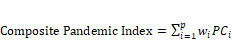(2).

   (2)

We use the scores of the first two extracted PCs and the weights are the proportion of variance accounted for by each PC as given in Table 4. For easy comparability with the stringency index, the composite measure of the pandemic is then calibrated on a scale of 0 to 100. For each observation or data point, we obtain a value of the index. Larger values of the pandemic index signify greater severity of the pandemic. The time path of this index is related to the movement of the stringency index. The stringency index is obtained from the Oxford COVID-19 Government Response Tracker (Hale et al., 2020). This index gives the stringency index values for each day and we collected the data from March 25, 2020, to May 15, 2021. The stringency index is a composite measure on a scale of 0 to 100 with 100 indicating highest stringency. It is based on nine response indicators such as school closures, workplace restrictions, and travel restrictions. It measures how the strictness of lockdown policies restricts movement and activities of people. Figure 3 gives the time-series graph of the constructed pandemic index and the stringency index from March 25, 2020, to May 15, 2021.

Figure 3. Time Series Plot of the Composite Pandemic Index and Stringency Index from March 25, 2020, to May 15, 2021

Source: Authors’ own (based on data obtained from Worldometer, Worldometers.info¹), and stringency index data obtained from Oxford COVID-19 Government Response Tracker (Hale et al., 2020).

In Table 5, the correlation coefficients between the pandemic index and the stringency index for the four different phases of the trajectory of the pandemic that are identified in the study are given. All the correlations coefficients are statistically significant. The overall estimated correlation coefficient for the entire period is –0.26385 indicating a negative relation between the pandemic and stringency index and this relation is statistically significant.

Table 5. Correlation Coefficients Between the Pandemic Index and the Stringency Index by Sub-periods

Source: Authors’ own (based on data obtained from Worldometer, Worldometers.info¹), and stringency index data obtained from Oxford COVID-19 Government Response Tracker (Hale et al., 2020).

  Figure 3 shows that when the stringency index (String. Index) value was high between March 25, 2020 (index was 100 on this date) and June 9, 2020, the pandemic index (Pand. Index) was initially zero and shows a very marginal increase in response to limited relaxations. The correlation coefficient is –0.73955 for this period. From June 10, 2020, till September 16, 2020, as the stringency index declined the pandemic index shows a quick increase and the correlation coefficient is –0.88047 for this period. Thus, until mid-September, we find a negative relationship between the two indices with the pandemic index increasing as stringency declined. Figure 3 also shows the puzzling phenomenon between mid-September 2020 and mid-February 2021 when, even though the stringency index declined the pandemic index also declined slowly and leveled off. The correlation coefficient for this period is 0.62107. Finally in the fourth phase, as the second wave of infections began, the pandemic index increased slowly in March 2021 and very rapidly in April 2021. In response, the stringency index also rose as many states imposed lockdowns and restrictions to curb transmission of the virus. The correlation coefficient is 0.85861 for this period. Thus in the last two phases, the correlation coefficient is positive with both indices moving in the same direction-either both declining or both increasing. The trend in the composite measure of the pandemic index also shows that the scale of the second wave of infections is significantly far more severe as compared to the first wave.

  The analysis of the trajectory of the pandemic by the different phases helps us establish the relation between path of the pandemic and its relation to the stringency index. The stringent lockdown on March 25, 2020, with the stringency index value of 100 was an ex-ante measure designed to prevent transmission, save lives and give the country time to put in place health systems to cope with the pandemic. The rise in the stringency index during the second wave is more a response to the sudden severity of the second wave of infections.

Discussion

From the health perspective, India seemed to have reaped the “lockdown dividend” in terms of lives saved. The Economic Survey of 2020–2021 estimates that the lockdown restricted COVID-19 spread by 3.7 million cases and saved more than 100,000 lives (Government of India [GoI], 2021a).

  Other statistical approaches to evaluating India’s lockdown policies on incidence rate using time-series approach also show that lockdown policy in India reduced incidence rate and helped “flatten the curve” buying additional time for pandemic preparedness (Thayer et al., 2021).

  The stringent lockdown saved lives but there was a cost in terms of loss of livelihoods. The economy contracted by a sharp 24.4% in the first quarter of fiscal year 2021 following the nationwide lockdown. This was the short-term pain that India was prepared to pay for saving human lives according to the Economic Survey (GoI, 2021a). The revival of the economy was planned through a number of sequenced policies to boost demand including a targeted stimulus program and complementary supply-side policies (GoI, 2021a; Goyal, 2020). Studies have shown that prompt and timely interventions can save lives with a not too significant cost in terms of foregone economic activity (Balmford et al., 2020). But for developing countries like India with a predominantly rural population, a large informal sector, and a high proportion of self-employed and casual labor, the stringent lockdown imposed a harsh and disproportionate burden on the most vulnerable sections of population pushing millions of people deeper into poverty (Biswas et al., 2020; International Labour Organization, 2020; Ray & Subramanian, 2020). Deprived of work and a livelihood the lockdown stranded many millions of people in cities away from their homes leading to an unprecedented crisis (Nayyar, 2020).

  Once the unlock phase began in June 2020, the economy showed signs of a recovery. With all key indicators improving, the Economic Survey of 2020–2021 (GoI, 2021a) pointed to a V-shaped recovery with a 7.5 % contraction in second quarter as compared to a 24% contraction in first quarter of 2021, and real GDP was expected to grow by 11% in fiscal year 2021–2022. Also, the pandemic situation which initially worsened in the unlock phase began showing a turnaround after mid-September 2020. From mid-September 2020 to mid-February 2021 it seemed that India was in a fortunate situation with the economy picking up and the scale of the pandemic showing a remarkable easing. The leftward inversion of the scatter of points in Figure 2 after mid-September points to a puzzling decline in the scale of the pandemic even as unlock measures continued leading many to believe that the pandemic was coming to an end in India (Biswas, 2021). The relative easing of the pandemic situation led to relaxation of many stringency measures. The Oxford Severity Index which was 100 as of March 25, 2020, steadily fell to 63.53 on March 1, 2021. But with relaxations continuing, the index fell further to its lowest level of 57.87 on April 1, 2021, even as coronavirus cases steadily increased after mid-February 2021. Given the epidemiological characteristics of new variants of the virus which had greater transmissibility, the imminent threat of a second wave was dormant and when it erupted suddenly in April 2021 it led to a serious health crisis (The Lancet, 2021). The magnitude and severity of the second wave points to the vital role of genomic surveillance as an integral part of pandemic management (Chakraborty et al., 2021; Cyranoski, 2021).

  Formulating and adopting policies to balance health and economy are crucial especially in the context of the second wave and possible future waves of infections. From the experience of the first wave, it would seem that rather than countrywide lockdowns, restrictions should instead be imposed at the state/local level where infections and positivity rates are high. The public health crisis in many cities in India during the second wave has led many states to impose restrictions in varying degrees of stringency (Sharma, 2021). The Oxford Stringency Index for India increased from 57.87 on April 1, 2021, to 73.61 on April 30, 2021, and increased further to 81.94 by May 10, 2021.

  The current high levels of infection in the second wave and the restrictions imposed by states to contain the transmission of the virus are likely to have an adverse impact on the economy (S&P Global Ratings, 2021). Although the Monthly Economic Review for April 2021 (GoI, 2021b) is optimistic that the effect on the economy may not be so severe as businesses have shown resilience in coping with COVID-19. Going forward, it may be useful to rely on data-driven policies that can identify at the state or local level as to which sectors or businesses need to have restrictions or shuttering. This can lead to informed decision-making so as to achieve public health goals and minimize social costs (Benzell et al., 2020).

  The challenges to containing the pandemic are many (Ajmera et al., 2020). While the vaccination program has begun in India, the task of vaccinating a population of over 1.3 billion people in India will take time and in the meantime policies for pandemic containment and management are important. Comprehensive testing of people and epidemiological tracking of new variants of coronavirus need to take primacy in these policies. Widespread acceptance and adoption of COVID-19 protocols at the individual level are essential to contain the spread of the virus (Newbold et al., 2020). And swiftly adopted and implemented government policies including expanding health systems and strengthening social protection systems are needed to reduce mortality rates and lessen the social and economic burden on people (Bigiani et al., 2020; Martinez-Valle, 2021).

Conclusion

During the last year, the spread of the COVID-19 pandemic has been closely followed. Using data on six dimensions of the pandemic the study used PCA to assess the trajectory of the pandemic in India in the two-dimensional space. The analysis enables us to visualize the path of the pandemic and identify four phases in the trajectory corresponding to the lockdown and unlock periods.

  Using the two extracted principal components, a composite pandemic index is constructed and its relation to the stringency index is examined. Overall the relation between the composite index of the pandemic and the stringency index was found to be negative and statistically significant. But the phase-wise analysis is significant for understanding the trajectory of the pandemic and lockdown policy. It reveals that the early stringent lockdown did help to save lives and push back the peak of the pandemic. But the puzzling and unexplained easing of the pandemic situation even as restrictions were eased between mid-September 2020 and mid-February 2021 and the suddenness and severity of the second wave of infections points to the need to track new variants of the virus for their transmissibility. Such epidemiological surveillance is vital for informed public health policy response to keep transmission levels low and save lives.

  The present study examines the relation between stringency measures and the path of the pandemic at an aggregative level but further research into the causal factors in the relation is needed. While the study covers a long duration of the pandemic and offers insights into the trajectory, it is clear from the second wave that managing the pandemic at local level is crucial. The significant variation in the spread of the pandemic across states in India indicates that further research using state or district level data needs to focus on the determinants of the spread of the pandemic, stringency measures adopted at the local level, and impact on mobility and local economy and business. Such district-level and state-level analysis can give insights into mitigation strategies for curtailment and management of possible future waves of infections.

Declaration of Conflicting Interests

The author declared the following potential conflicts of interest with respect to the research, authorship, and/or publication of this article: This research work has not been published elsewhere in the same form nor has it been sent for consideration for publication elsewhere.

Funding

The author received no financial support for the research, authorship, and/or publication of this article.

Note

1.  https://www.worldometers.info/coronavirus/country/india/